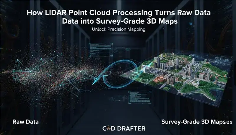
LiDAR Point Cloud Processing: How Raw Data Are Transformed into Survey-Grade 3D Maps

A huge myth about the surveying and mapping sector is that LiDAR scanners do not produce 3D maps. A drone or a scanner on the ground does not print out a gorgeous, color-coded 3D model that you can drop into your CAD software when it is finished with its run.

Rather, it creates a huge, disorganized, and entirely incomprehensible swarm of digital dots referred to as raw point clouds. To give you some idea of the scale, a contemporary scanner of the earth (such as the Leica RTC360) is able to scan more than 200 million points within 90 seconds.

It takes a very complex computational pipeline to transform that digital snowstorm into an actionable, accurate 3D map. This processing pipeline will be more precise and quicker than ever in 2026 due to the combination of cloud, AI-based semantic segmentation, and sophisticated filtering algorithms.

To know how we can convert billions of blind data points and map precision engineering, you must know the matrix. We can start with deconstructing the process of modern LiDAR point cloud processing.

What Is a Raw Point Cloud?

We have to know what is being recorded by the scanner before we can process the data.

When the LiDAR sensor emits a burst of light (a laser pulse) on an object, it bounces back to the sensor. The system records the exact time that the light returned, and the distance is reckoned. This is done millions of times per second.

However, a raw point cloud is not only a set of distances. Each of the 200 million points of such data has a number of key attributes:

• Spatial Coordinates (X, Y, Z): The precise position of the point in space (typically with reference to a global GNSS (Global Navigation Satellite System) positioning system).
• Intensity: It is a measure of the strength of the signal of the return. Various media have different light reflections. A street sign with a large intensity value will be the one that is highly reflective, whereas a dark asphalt will be the one with a very small intensity value. This is very important in the identification of materials later.
• Return Number: One laser pulse may strike several objects. As an example, a pulse may strike a tree branch (Return 1), puncture through the leaves to strike a lower bush ( Return 2), and finally strike the ground ( Return 3). It is the ability to capture several returns that enables LiDAR to be able to look through vegetation.
• Color (RGB/NIR): In several LiDARs developed in recent times, a high-resolution camera is attached that assigns a true color or Near-Infrared value to each point in real time.

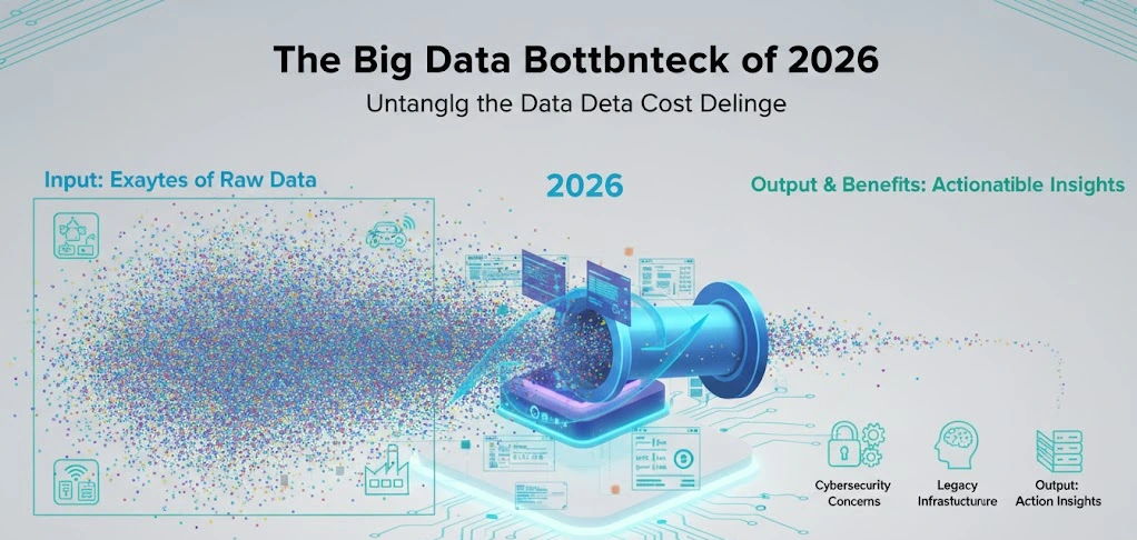
The Big Data Bottleneck of 2026

This data is so resource-intensive to process. A standard airborne LiDAR scan of the city scale can scale to multiple terabytes of raw data with ease. To reduce such large files the industry is currently heavily depending on advanced edge-to-cloud architectures (such as AWS DataSync) and real-time neural compression algorithms (such as RENO – Real-Time Neural Compression) to compress these large files without loss of geometry, enabling field teams to upload them to cloud servers to be heavily-computed.

The Point Cloud Processing Pipeline

The process of converting the raw digital clay to a finalized 3D map or Digital Elevation Model (DEM) is a highly rigorous, multi-stage process. One step more, and your millimeter-precise survey will become a contorted, useless thing.

Step 1: Registration and Alignment 

A LiDAR scanner is not able to scan a building from a single point. The scanner will be scanned at dozens (or hundreds) of various set-up positions by the surveyor, to ensure that all the angles are recorded, and no shadows (blind spots) are present. Drones are doing this in the course of their flight.

The mathematical process of moving these individual, overlapping masses of point clouds and joining them up into a single global coordinate system is the very first step in processing, which is called Registration.

SLAM (Simultaneous Localization and Mapping): 

SLAM algorithms can be used to follow the path of the scanner in real-time by mobile / backpack LiDAR systems that traverse GPS-denied regions (such as dense forests or underground mines). It takes advantage of the geometry of the cloud-based CAD drafting itself to determine the movement of the scanner.

The ICP Algorithm: 

The best algorithm to use when refining this alignment is the Iterative Closest Point (ICP) algorithm. The software compares two overlapping scans and finds out the similarities in the geometric attributes (such as the corners of a room) in the scans and then mathematically rotates and translates one scan until there is a minimum distance between the similar points.

You will get ghosting in case the registration is off by even a fraction of a degree. That means it will make the walls seem twice their proper thickness, and pipes appear to be cut in two.

 

Step 2: Pre-Processing, Filtering, and Reduce Noise (Cleaning the Chaos)

Now that the world has been patched up, it is time to clean up the mess. LiDAR sensors are very delicate. They not only seize structures and landscape, but they also seize birds flying overhead, dust in the air, rain, walking bodies in the frame and sensor noise.

This is undesirable information and is known as Noise, which should be ruthlessly removed.

Voxel Downsampling

A surveyor had to stand in one place too long, as there could be 50 000 points squeezed into a square inch of a wall. Such over-density kills software and gives no concrete details. Voxel Downsampling is used by processors.

The software subdivides the 3D space into small 3D cubes (voxels). In the case of a voxel having 500 points, the algorithm will be used to compute the center of mass of the points, and will substitute them with one high-quality representative point. This significantly compresses the size of the file without losing the geometric shape.

Statistical Outlier Removal (SOR)

What makes a computer distinguish between a real object and the glitch of the sensor? Through the analysis of the neighborhood.

The SOR algorithm examines one point and evaluates the distance between the point and its closest neighbors. When a point is floating in the air, distant in any way to another group of points (such as a bird or a raindrop), the algorithm marks it as an outlier and removes it.

Guided Point Cloud Filtering

In complex environments like dense forests, advanced 2026 algorithms use “guided filtering” based on linear models. This ensures that while noise is removed, critical sharp geometric features (like the exact edge of a building or the diameter of a tree trunk) are perfectly preserved, drastically reducing the Root Mean Square Error (RMSE) of the final map.

Raw Data vs. Processed LiDAR Data

Feature	Raw LiDAR Point Cloud	Processed & Filtered Point Cloud
Data Size	Massive (100GB – 1TB+)	Optimized & Downsampled (10GB – 50GB)
Coordinate System	Local (Relative to the scanner)	Global (Tied to GNSS/Real-world coordinates)
Noise Level	High (Includes birds, dust, reflections, ghosts)	Low (Outliers and statistical anomalies removed)
Density	Uneven (Hyper-dense near scanner, sparse far away)	Uniform (Normalized via voxel downsampling)
Usability	Unusable in standard CAD/BIM software	Ready for Classification and 3D Modeling

Step 3: Semantic Classification (Giving the Data a Brain)

So far, the computer only perceives a perfectly clean and aligned set of points. But it is still “dumb” data. The computer does not know that a cluster of points is a maple tree, and that cluster of points is an asphalt road.

This leads to the most computationally intensive and exciting step of the 2026 processing pipeline:

Classification

The classification is the procedure of giving a particular name (or a category) to each and every point. The American Society of Photogrammetry and Remote Sensing (ASPRS) contains standard classification codes (e.g, Class 2 Ground, Class 6 Buildings, Class 3 Low Vegetation).

The Transition between Rules and AI

Classification was rule-based a few years ago. We employed such algorithms as Progressive Morphological Filter (PMF) or Cloth Simulation Filter (CSF).

• The mechanism of CSF: Visualize the point cloud and flip it upside down. Then place a digital piece of cloth on the cloud. The textile covers the “peaks” (but in fact the lowest points of the terrain, as it is in inverted form). Any point that lies on the cloth is considered to be Bare Earth. Any point that is below the cloth is considered as Vegetation or Building.

Although these geometric rules remain in use to extract bare-earth Digital Terrain Models (DTMs), the industry has strongly switched to the use of Open Source Cad Software, Machine Learning, and Deep Learning (Semantic Segmentation).

The result of this AI integration is that, with only a few button presses, a multi-million point dataset can be categorized into complex sub-categories instantly: not just between a tree and a building, but between an oak tree, a power line, a streetlamp, and a fire hydrant, with near-perfect accuracy.

Get accurate, survey-grade 3D maps from raw LiDAR data with trusted professional processing!

Step 4: Feature Extraction and Vectorization (Joining the Digital Dots)

And thus your point cloud is perfectly aligned, washed of noises, and sorted into distinct classes by an AI. The computer has been made aware of the dots that are the ground and the dots that are a building.

However, this is still not easily importable into normal CAD software, such as AutoCAD or Revit, and supposedly functions as a building. Dots are not used in building by engineers. They are constructed using lines, polygons, cylinders, and solid surfaces.

This is where we enter the world of data visualization/engineering reality. We pass into the stage of Feature Extraction and Vectorization.

This algorithm accepts the categorized groups of points and geometrically fits them with geometric shapes.

• Plane Fitting: When the algorithm identifies a huge, flat, vertical grouping of points that is defined as a Building, it applies algorithms such as RANSAC (Random Sample Consensus) to compute the ideal mathematical plane that goes through those points. A million dots turn in a second into a perfectly smooth wall.
• Cylinder Fitting: A point cloud of a refinery in industrial surveying is nothing more than a spaghetti-bowl of dots. The software identifies points that are categorized as Piping, computes the curvature of the points and substitutes them with an ideal 3D cylinder made of solid. It even figures the exact pipe diameter and the centerline.
• Edge Detection: To trace a property line or an edge of a curb, the application searches for abrupt decreases in altitude or a sharp shift in the point normals (the direction the points are facing). It automatically attracts a vector polyline along such an edge.

Automated Scan-to-BIM (Building Information Modeling), is the sacred grail of this process in 2026. Rather than a human draughtsman manually tracking 40 hours to trace the points, deep learning algorithms are used to automatically identify doors, windows, structural beams, and HVAC ductwork and transform the point cloud into an intelligent, parametric 3D model within seconds.

Step 5: Surface Generation (The Art of the Bare Earth)

To the civil engineers, surveyors and hydrologists, the building is not the most significant aspect of the scan. The ground is. They must be aware of how much water will be moved across a site, or how many cubic yards of dirt should be moved to level a foundation.

To accomplish this, whatever is not the ground (trees, cars, buildings) is removed in the processing pipeline, and the resulting surface is continuous.

This is achieved by the formation of TIN (Triangulated Irregular Network). The software then picks up all the points that are labeled as Ground and then makes lines between the closest neighbors and creates a huge, continuous web of triangles. This is basically a shrink wrapping of the ground points.

This step generates three very distinct, but critically important, types of maps:

DEM vs. DTM vs. DSM

Model Type	What It Stands For	What It Actually Shows	Primary Real-World Use Case
DSM	Digital Surface Model	The absolute top layer of everything. Includes the tops of trees, roofs of houses, and power lines.	Urban planning, line-of-sight analysis for telecommunications (5G cell towers), and aviation obstacle planning.
DTM	Digital Terrain Model	The “Bare Earth.” All vegetation and man-made structures are mathematically stripped away.	Flood modeling, road design, topographic surveying, and contour map generation.
DEM	Digital Elevation Model	A generic term often used interchangeably with DTM, representing a grid of elevation squares (raster).	Broad topographical mapping, volumetric calculations for mining and earthworks.

The ability to instantly toggle between a DSM (seeing the forest canopy) and a DTM (seeing the hidden ground beneath the forest) is the primary reason LiDAR completely replaced traditional photogrammetry for land surveying. A camera cannot see through leaves. A laser can.

Step 6: 3D Meshing and the 2026 “Gaussian Splatting” Revolution

If you want to show your LiDAR data to an engineer, you give them a vectorized CAD file. If you want to show it to an investor, a mayor, or the general public, you need to make it look flawlessly real.

Historically, this meant using algorithms like Poisson Surface Reconstruction to stretch a digital “skin” over the point cloud, and then pasting the RGB color data onto that skin to create a 3D textured mesh. It worked, but it was incredibly computationally heavy, and trees or thin structures like chain-link fences usually looked like melted plastic.

Welcome to 2026. The pipeline has been completely upended by 3D Gaussian Splatting (3DGS).

Instead of forcing points to become a solid mesh, 3DGS is a machine learning rendering technique. It takes the raw, colored LiDAR points and represents each point as a tiny, semi-transparent, mathematically optimized “splat” (like a microscopic drop of paint).

• Why it matters: An AI trains itself on how light passes through these splats. The result is a photorealistic, real-time 3D environment that can be rendered smoothly on a standard web browser or VR headset.
• The Result: Thin structures like powerlines remain perfectly sharp. Trees retain their complex, leafy transparency. The visual fidelity of the raw LiDAR scan is perfectly preserved without the “blocky” artifacts of traditional meshing.

In the modern processing pipeline, exporting a 3DGS file has become the gold standard for creating immersive Digital Twins of cities and infrastructure.

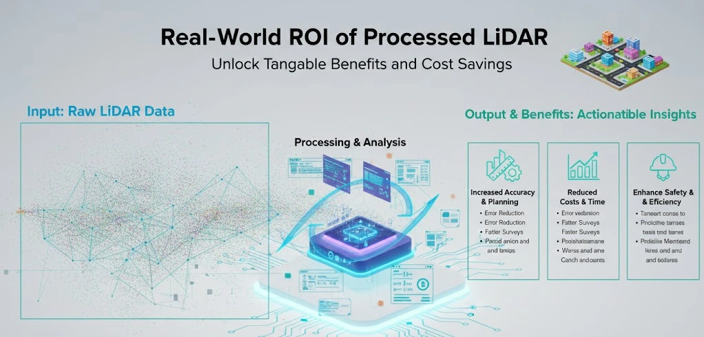
Real-World ROI of Processed LiDAR

We’ve walked through the matrix. We’ve aligned, filtered, classified, vectorized, and meshed the data. But why spend tens of thousands of dollars on scanning equipment and cloud computing to do this?

Because accurate spatial data is the most valuable currency in the physical world. Here is how this processed data is actively transforming global industries:

1. Construction and AEC (Clash Detection)

Imagine building a $400 million hospital retrofit. You have the original blueprints from 1985. You design your new HVAC system based on those prints. But during construction, you discover a massive structural beam was installed two feet to the left of where the blueprint says it should be. Your custom ductwork crashes into it.

Cost of the error: $150,000 and a 3-week delay.

If the site was laser-scanned first, the processed point cloud would reveal the exact, real-world, as-built conditions. Engineers overlay the new 3D design onto the processed point cloud to perform Clash Detection, identifying collisions digitally before a single piece of steel is cut.

2. Forestry and Biomass Calculation

In the fight against climate change, we need to know exactly how much carbon is stored in our forests. You can’t put a forest on a scale.

Instead, drones fly LiDAR over the canopy. The processing pipeline separates the ground (DTM) from the canopy (DSM) to create a Canopy Height Model (CHM). Advanced algorithms then identify individual tree crowns, count the trees, measure their height, and estimate the exact trunk diameter. From this, environmental scientists can calculate the precise biomass and carbon-capture value of a million acres of timber in a matter of hours.

3. Disaster Mitigation and Flood Modeling

When a hurricane approaches the coast, emergency planners don’t guess where the water will go. They rely on processed LiDAR DTMs.

By stripping away the buildings and trees, hydrologists run fluid-dynamics simulations over the bare-earth model. Because the LiDAR data is accurate down to the centimeter, they can predict exactly which streets will flood, which retaining walls will fail, and which neighborhoods need mandatory evacuation orders.

4. Autonomous Vehicles and HD Mapping

A self-driving car doesn’t just use its onboard sensors to see the road; it relies on a pre-processed HD Map (High-Definition Map). Mobile LiDAR scanners mount to vehicles and map the entire highway system. 

The point cloud processing pipeline automatically extracts the lane markings, measures the height of the overpasses, and maps the exact curvature of the guardrails. The car compares its live sensor data against this pre-processed map to know its location down to the millimeter, even in a blinding snowstorm.

Frequently Asked Questions

If LiDAR sees in points, how does it penetrate dense forest canopies?

It’s all about the Multiple Return capability. A single laser pulse isn’t stopped by the first leaf it hits. Instead, the beam splits; part of the energy bounces off the top branch (Return 1), while the rest travels deeper to hit a lower bush (Return 2), finally reaching the forest floor (Return 3). Processing algorithms then strip away the first few returns to reveal the hidden topography beneath the trees.

Why can’t I just upload raw scan data directly into AutoCAD or Revit?

Raw point clouds are essentially “unintelligent” clusters of billions of coordinates. Standard CAD software is built to handle vector geometry (lines, arcs, and planes), not a massive “digital blizzard of dots. Without processing steps like feature extraction and vectorization, your computer would likely crash attempting to render the sheer volume of unorganized data.

What is “Ghosting,” and why does it ruin survey accuracy?

Just like other common CAD drafting mistakes, Ghosting occurs when the Registration phase fails. If two overlapping scans aren’t aligned to the millimeter, the same wall will appear in two slightly different positions. This creates a visual “double image” where structures look unnaturally thick or pipes appear to split. In engineering, this leads to catastrophic errors in clash detection.

How does AI-driven Semantic Segmentation differ from old-school filtering?

Old-school methods relied on rigid geometric rules, like “if it’s high off the ground, it’s a tree. AI changes the game by analyzing neighborhood statistics. In 2026, neural networks recognize the signature of an object, distinguishing a power line from a tree branch based on the intensity of the reflection and the mathematical “roughness” of the point cluster.

Is there a difference between a DTM and a DSM?

Yes, and the distinction is vital for civil engineering. A Digital Surface Model (DSM) captures the “first return” of everything. A Digital Terrain Model (DTM) is the “Bare Earth” version; it’s the result of processing that mathematically “mows the grass” and removes buildings to show only the true soil elevation.

What is 3D Gaussian Splatting, and is it better than traditional meshing?

Traditional meshing stretches a “skin” over points, which often looks like melted plastic on thin objects. 3D Gaussian Splatting (3DGS) is a 2026 breakthrough that represents points as tiny, semi-transparent mathematical “splats.” This allows for photorealistic, high-speed rendering that keeps power lines sharp and trees looking transparent and natural in a digital twin.

How does Voxel Downsampling save my computer from crashing?

A scanner might capture 50,000 points on a single square inch of a wall near the tripod. This is redundant data. Voxel Downsampling creates a 3D grid of tiny cubes (voxels) and collapses all points within a cube into one single, mathematically averaged point. You keep the exact shape of the wall but reduce the file size by up to 90%.

Can LiDAR data be used for volumetric calculations in mining?

Absolutely. By comparing a DTM of a site before and after an excavation, software can calculate the exact volume of material moved. Because LiDAR is accurate to the centimeter, these “cut and fill” calculations are far more precise than traditional manual surveying, saving mining companies millions in logistics costs.

Conclusion

A LiDAR scanner is a magnificent piece of hardware. But hardware alone is completely blind.

The true magic of 3D mapping doesn’t happen in the field; it happens in the cloud. It happens in the rigorous, mathematically punishing steps of registration, noise reduction, semantic segmentation, and vectorization.

As we push deeper into 2026, the volume of spatial data is exploding. With the integration of deep learning AI and real-time processing architectures, we are no longer just making maps. We are building 1:1 digital replicas of reality.

The next time you look at a flawless 3D model of a city, a factory, or a landscape, remember what you are actually looking at. You aren’t looking at a photograph. You are looking at billions of chaotic, digital dots that were wrestled into order by one of the most sophisticated computational pipelines ever created.